PIPR preprocessing pipeline

What follows is an example pipeline for preprocessing PIPR data with tools from pyplr.utils and pyplr.preproc. The data were collected from three subjects using this protocol.

import os.path as op

import pandas as pd
import matplotlib.pyplot as plt
import seaborn as sns
sns.set_context('notebook', font_scale=1.2)

from pyplr import graphing, utils, preproc
from pyplr.plr import PLR

# Some useful constants
SAMPLE_RATE = 120
DURATION = 7800
ONSET_IDX = 600

# Columns to load
use_cols = ['confidence',
            'method',
            'pupil_timestamp',
            'eye_id',
            'diameter_3d',
            'diameter']

# Pupil Labs recording directories / exports
subjects = {
    '001': [r'/Users/jtm/Projects/PyPlr/examples/PIPR/data/sub001', '000'],
    '002': [r'/Users/jtm/Projects/PyPlr/examples/PIPR/data/sub002', '001'],
    '003': [r'/Users/jtm/Projects/PyPlr/examples/PIPR/data/sub003', '000']
}

# Empty DataFrame to store processed PIPR data
df = pd.DataFrame()

# Loop over subjects
for k in subjects.keys():
    # Get a handle on a subject
    rec = subjects[k][0]
    export = subjects[k][1]
    s = utils.new_subject(
        rec, export=export, out_dir_nm='pyplr_analysis')

    # Load pupil data
    samples = utils.load_pupil(
        s['data_dir'], eye_id='best', method='3d', cols=use_cols)

    # Pupil columns to analyse
    pupil_cols = ['diameter_3d', 'diameter']

    # Make figure for processing
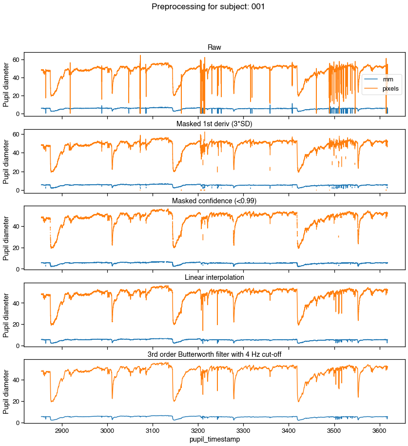
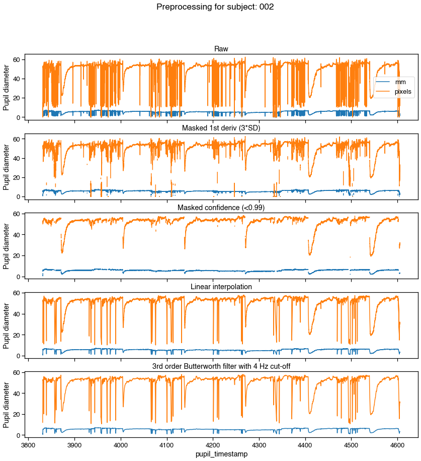
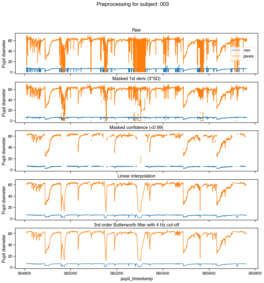
    f, axs = graphing.pupil_preprocessing(nrows=5, subject=k)

    # Plot the raw data
    samples[pupil_cols].plot(title='Raw', ax=axs[0], legend=True)
    axs[0].legend(loc='center right', labels=['mm', 'pixels'])

    # Mask first derivative threshold
    samples = preproc.mask_pupil_first_derivative(
        samples, threshold=3.0, mask_cols=pupil_cols)
    samples[pupil_cols].plot(
        title='Masked 1st deriv (3*SD)', ax=axs[1], legend=False)

    # Mask confidence threshold
    samples = preproc.mask_pupil_confidence(
        samples, threshold=0.99, mask_cols=pupil_cols)
    samples[pupil_cols].plot(
        title='Masked confidence (<0.99)', ax=axs[2], legend=False)

    # Interpolate
    samples = preproc.interpolate_pupil(
        samples, interp_cols=pupil_cols)
    samples[pupil_cols].plot(
        title='Linear interpolation', ax=axs[3], legend=False)

    # Smooth with Butterworth filter
    samples = preproc.butterworth_series(
        samples, fields=pupil_cols, filt_order=3,
        cutoff_freq=4/(SAMPLE_RATE/2))
    samples[pupil_cols].plot(
        title='3rd order Butterworth filter with 4 Hz cut-off',
        ax=axs[4], legend=False)

    # Load events
    events = utils.load_annotations(s['data_dir'])

    # Extract the event ranges
    ranges = utils.extract(
        samples,
        events,
        offset=-ONSET_IDX,
        duration=DURATION,
        borrow_attributes=['color'])

    # Calculate baselines
    baselines = ranges.loc[:, range(0, ONSET_IDX), :].mean(level=0)

    # New columns for percent signal change
    ranges = preproc.percent_signal_change(
        ranges, baselines, pupil_cols)

    # Add to DataFrame
    ranges['Subject'] = k
    df = df.append(ranges)

    # Convert samples index-level to time (s)
    new_onset = (ranges.index.get_level_values('onset')
                       .unique()
                 - ONSET_IDX) / SAMPLE_RATE
    ranges.index = ranges.index.set_levels(
        levels=new_onset, level='onset')
    ranges.to_csv(op.join(s['out_dir'], 'ranges.csv'))

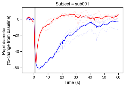
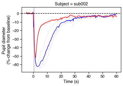
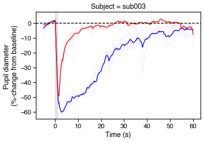
    # Plot PIPRs
    fig, ax = plt.subplots(figsize=(6,4))
    for r in range(6):
        c = ranges.loc[r, 'color'][0]
        ranges.loc[r, 'diameter_pc'].plot(
            color=c, lw='.1', ax=ax, legend=False)

    # Now show the means
    avgs = (ranges.reset_index()
                  .groupby(['color','onset'], as_index=False)
                  .mean())
    sns.lineplot(data=avgs, x='onset', y='diameter_pc', hue='color',
                 palette={'blue':'b','red':'r'}, legend=False)

    # Tweak figures
    ax.axvspan(0, 1, color='k', alpha=.1)
    ax.axhline(0, 0, 1, color='k', ls='--')
    ax.set_xlabel('Time (s)')
    ax.set_ylabel('Pupil diameter \n(%-change from baseline)')
    ax.set_title('Subject = {}'.format(s['id']))

    # Save
    fig.savefig('../img/PIPR_{}.svg'.format(s['id']))

# Save Processed PIPR data
df.to_csv('processed_PIPR.csv')

************************************************************
************************** sub001 **************************
************************************************************
Loaded 94406 samples
Loaded 6 events
Extracted ranges for 6 events
************************************************************
************************** sub002 **************************
************************************************************
Loaded 95307 samples
Loaded 6 events
Extracted ranges for 6 events
************************************************************
************************** sub003 **************************
************************************************************
Loaded 117246 samples
Loaded 6 events
Extracted ranges for 6 events