Analysis of pupil data

There are many valid approaches to the analysis of pupillometry data, but the optimal approach will depend on the type of experiment being run and the research question in mind. Kelbsch et al. (2019) provide an informative view on standards in pupillometry, and there are some great examples of community-developed packages for streamlining pupillometry data analysis. Whilst it is always worth exploring the wider options that are available, PyPlr includes a set of pandas-reliant (you won’t regret learning pandas!) scripting tools for implementing a standard data processing pipeline that is optimised to work with some of the idiosynchrasies of Pupil Labs data. So far we have found these tools to be adequate for analysing our own data, but we welcome suggestions for improvements.

See here for a general introduction to analysing Pupil Labs pupillometry data. What follows is a typical PyPlr analysis pipeline with tools from pyplr.utils and pyplr.preproc.

Export with Pupil Player

The first step in our pipeline is to export the data using Pupil Player, making sure the required plugins (e.g., Annotation Player plugin) are enabled. Currently this must be done individually for each recording. Below is printed the file structure of a typical recording after export (more info on recording format here).

from pyplr import utils

# Pupil Labs recording directory
rec_dir = '/Users/jtm/OneDrive - Nexus365/protocols/pipr_protocol/JTM'
utils.print_file_structure(rec_dir)

JTM/
    .DS_Store
    annotation.pldata
    annotation_player.pldata
    annotation_player_timestamps.npy
    annotation_timestamps.npy
    blinks.pldata
    blinks_timestamps.npy
    eye1.intrinsics
    eye1.mp4
    eye1_lookup.npy
    eye1_timestamps.npy
    fixations.pldata
    fixations_timestamps.npy
    gaze.pldata
    gaze_timestamps.npy
    info.player.json
    notify.pldata
    notify_timestamps.npy
    pupil.pldata
    pupil_timestamps.npy
    surface_definitions_v01
    user_info.csv
    world.intrinsics
    world.mp4
    world_lookup.npy
    world_timestamps.npy
    analysis/
        plr_extraction.png
        plr_metrics.csv
        plr_overall_metrics.png
        processed.csv
        pupil_processing.png
    exports/
        000/
            annotations.csv
            export_info.csv
            gaze_positions.csv
            pupil_gaze_positions_info.txt
            pupil_positions.csv
            world.mp4
            world_timestamps.csv
            world_timestamps.npy
    pyplr_analysis/
    offline_data/
        tokens/
            gaze_positions_consumer_Vis_Polyline.token
            gaze_positions_producer_GazeFromRecording.token
            pupil_positions_consumer_Pupil_From_Recording.token
            pupil_positions_consumer_System_Timelines.token
            pupil_positions_producer_Pupil_From_Recording.token

Load exported data

Now we can set up some constants and use pyplr.utils to get things moving. new_subject(...) returns a dictionary with the root directory, recording id, data directory and a newly made output directory for the analysis results. Then, passing the data directory to load_pupil(...), we load the specified columns from the pupil_positions.csv exported data.

# Columns to load
use_cols = ['confidence',
            'method',
            'pupil_timestamp',
            'eye_id',
            'diameter_3d',
            'diameter']

# Get a handle on a subject
s = utils.new_subject(
    rec_dir, export='000', out_dir_nm='pyplr_analysis')

# Load pupil data
samples = utils.load_pupil(
    s['data_dir'], eye_id='best', cols=use_cols)
samples

************************************************************
*************************** JTM ****************************
************************************************************
Loaded 48552 samples

	eye_id	confidence	diameter	method	diameter_3d
pupil_timestamp
85838.895658	1	0.977211	50.102968	3d c++	6.105771
85838.903656	1	0.997867	50.037086	3d c++	6.099682
85838.911644	1	0.998295	49.702628	3d c++	6.060059
85838.919551	1	0.997833	49.968637	3d c++	6.093759
85838.927504	1	0.998183	49.883191	3d c++	6.084404
...	...	...	...	...	...
86246.730916	1	0.818574	56.684975	3d c++	6.966634
86246.739307	1	0.947873	56.824819	3d c++	6.983579
86246.746889	1	0.969337	57.176728	3d c++	7.027931
86246.758588	1	0.956524	56.838490	3d c++	6.988390
86246.762987	1	0.927155	56.933094	3d c++	7.000156

48552 rows × 5 columns

Preprocessing

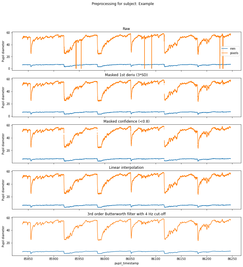
Preprocessing pupillometry data is relatively straight-forward and typically involves dealing with signal loss due to eye blinks and smoothing out any high frequency noise. There are sophisticated algorithms for detecting blinks in a pupil time course, but Pupil Player has its own Blink Detection plugin that detects blinks based on rapid changes in the confidence metric. Whilst you can export these blink events and use the timestamps to index and mask the pupil timecourse, we find that it is effective simply to mask the pupil data with thresholds on the first derivative and confidence metric, and then to follow up with linear interpolation and smoothing.

from pyplr import graphing
from pyplr import preproc

# Sampling frequency
SAMPLE_RATE = 120

# Pupil columns to analyse
pupil_cols = ['diameter_3d', 'diameter']

# Make figure for processing
f, axs = graphing.pupil_preprocessing(nrows=5, subject='Example')

# Plot the raw data
samples[pupil_cols].plot(title='Raw', ax=axs[0], legend=True)
axs[0].legend(loc='center right', labels=['mm', 'pixels'])

# Mask first derivative
samples = preproc.mask_pupil_first_derivative(
    samples, threshold=3.0, mask_cols=pupil_cols)
samples[pupil_cols].plot(
    title='Masked 1st deriv (3*SD)', ax=axs[1], legend=False)

# Mask confidence
samples = preproc.mask_pupil_confidence(
    samples, threshold=0.8, mask_cols=pupil_cols)
samples[pupil_cols].plot(
    title='Masked confidence (<0.8)', ax=axs[2], legend=False)

# Interpolate
samples = preproc.interpolate_pupil(
    samples, interp_cols=pupil_cols)
samples[pupil_cols].plot(
    title='Linear interpolation', ax=axs[3], legend=False)

# Smooth
samples = preproc.butterworth_series(
    samples, fields=pupil_cols, filt_order=3,
    cutoff_freq=4/(SAMPLE_RATE/2))
samples[pupil_cols].plot(
    title='3rd order Butterworth filter with 4 Hz cut-off',
    ax=axs[4], legend=False);

Extraction

Having cleaned the timecourse we need to extract the events of interest. This requires the annotation events sent during the recording, which have the timestamps needed for extraction. These can be loaded with utlis.load_annotations(...).

events = utils.load_annotations(s['data_dir'])
events

Loaded 6 events

	index	label	duration	color	creation_time	creator	protocol	pulse_duration	pulse_spec
timestamp
85854.348667	1835	LIGHT_ON	NaN	red	2020-11-10 09:39:10.888989	jtm	pulse	1000	[0, 0, 0, 0, 0, 0, 0, 0, 0, 1979]
85919.820362	9629	LIGHT_ON	NaN	blue	2020-11-10 09:39:10.882007	jtm	pulse	1000	[0, 0, 0, 2500, 0, 0, 0, 0, 0, 0]
85985.280630	17422	LIGHT_ON	NaN	blue	2020-11-10 09:39:10.882007	jtm	pulse	1000	[0, 0, 0, 2500, 0, 0, 0, 0, 0, 0]
86050.768628	25217	LIGHT_ON	NaN	red	2020-11-10 09:39:10.888989	jtm	pulse	1000	[0, 0, 0, 0, 0, 0, 0, 0, 0, 1979]
86116.228025	33008	LIGHT_ON	NaN	blue	2020-11-10 09:39:10.882007	jtm	pulse	1000	[0, 0, 0, 2500, 0, 0, 0, 0, 0, 0]
86181.688172	40801	LIGHT_ON	NaN	red	2020-11-10 09:39:10.888989	jtm	pulse	1000	[0, 0, 0, 0, 0, 0, 0, 0, 0, 1979]

Now we can pass our samples and events to utils.extract(...) along with some parameters defining the number of samples to extract and how much to offset the data relative to the event. Here we extract-65 second epochs and offset by a 5 second baseline period.

# Number of samples to extract and which sample
# should mark the onset of the event
DURATION = 7800
ONSET_IDX = 600

# Extract the event ranges
ranges = utils.extract(
    samples,
    events,
    offset=-ONSET_IDX,
    duration=DURATION,
    borrow_attributes=['color'])
ranges

Extracted ranges for 6 events

		eye_id	confidence	diameter	method	diameter_3d	interpolated	orig_idx	color
event	onset
0	0	1.0	0.998989	48.404937	3d c++	5.990967	0	85849.311553	red
	1	1.0	0.998972	48.436117	3d c++	5.994949	0	85849.319757	red
	2	1.0	0.999134	48.469848	3d c++	5.999237	0	85849.327708	red
	3	1.0	0.998426	48.505896	3d c++	6.003802	0	85849.335675	red
	4	1.0	0.998895	48.544031	3d c++	6.008612	0	85849.343669	red
...	...	...	...	...	...	...	...	...	...
5	7795	1.0	0.922093	54.375155	3d c++	6.707360	0	86242.127040	red
	7796	1.0	0.977674	54.338056	3d c++	6.703963	0	86242.135026	red
	7797	1.0	0.933031	54.304633	3d c++	6.701016	0	86242.142965	red
	7798	1.0	0.970404	54.274990	3d c++	6.698505	0	86242.150957	red
	7799	1.0	0.903852	54.249187	3d c++	6.696413	0	86242.162996	red

46800 rows × 8 columns

utils.extract(...) returns a pandas DataFrame with a two-level (event, onset) hierarchichal index. The original index to the data is preserved in a column along with any attributes borrowed from the annotations. Now is a good time to create additional columns expressing the pupil data as percent signal change from baseline.

# Calculate baselines
baselines = ranges.loc[:, range(0, ONSET_IDX), :].mean(level=0)

# New columns for percent signal change
ranges = preproc.percent_signal_change(
    ranges, baselines, pupil_cols)
ranges

		eye_id	confidence	diameter	method	diameter_3d	interpolated	orig_idx	color	diameter_3d_pc	diameter_pc
event	onset
0	0	1.0	0.998989	48.404937	3d c++	5.990967	0	85849.311553	red	-6.907039	-7.009474
	1	1.0	0.998972	48.436117	3d c++	5.994949	0	85849.319757	red	-6.845173	-6.949574
	2	1.0	0.999134	48.469848	3d c++	5.999237	0	85849.327708	red	-6.778534	-6.884774
	3	1.0	0.998426	48.505896	3d c++	6.003802	0	85849.335675	red	-6.707607	-6.815521
	4	1.0	0.998895	48.544031	3d c++	6.008612	0	85849.343669	red	-6.632865	-6.742260
...	...	...	...	...	...	...	...	...	...	...	...
5	7795	1.0	0.922093	54.375155	3d c++	6.707360	0	86242.127040	red	8.891820	8.796684
	7796	1.0	0.977674	54.338056	3d c++	6.703963	0	86242.135026	red	8.836673	8.722455
	7797	1.0	0.933031	54.304633	3d c++	6.701016	0	86242.142965	red	8.788822	8.655579
	7798	1.0	0.970404	54.274990	3d c++	6.698505	0	86242.150957	red	8.748060	8.596268
	7799	1.0	0.903852	54.249187	3d c++	6.696413	0	86242.162996	red	8.714104	8.544640

46800 rows × 10 columns

Plotting and parametrisation

It is common practice when analysing the PLR to describe it in terms of paremeters relating to time, velocity and acceleration. So once you have an array of data representing a pupil’s response to light, be it from a single trial or an average of multiple trials, simply pass it to pyplr.plr.PLR along with some basic parameters.

from pyplr.plr import PLR

average_plr = ranges.mean(level=1)['diameter_3d'].to_numpy()
plr = PLR(average_plr,
          sample_rate=SAMPLE_RATE,
          onset_idx=ONSET_IDX,
          stim_duration=1)

Now you can do a quick plot with options to display the velocity and acceleration profiles and the derived parameters:

fig = plr.plot(vel=True, acc=True, print_params=True)

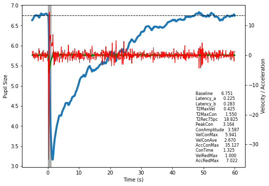
Or simply access the parameters as a DataFrame.

params = plr.parameters()
params

	value
Baseline	6.751031
Latency_a	0.225000
Latency_b	0.283333
T2MaxVel	0.425000
T2MaxCon	1.550000
T2Rec75pc	18.825000
PeakCon	3.164023
ConAmplitude	3.587008
VelConMax	5.940593
VelConAve	2.670336
AccConMax	35.127363
ConTime	1.325000
VelRedMax	0.999670
AccRedMax	7.021978